Approach | thereiswaldo

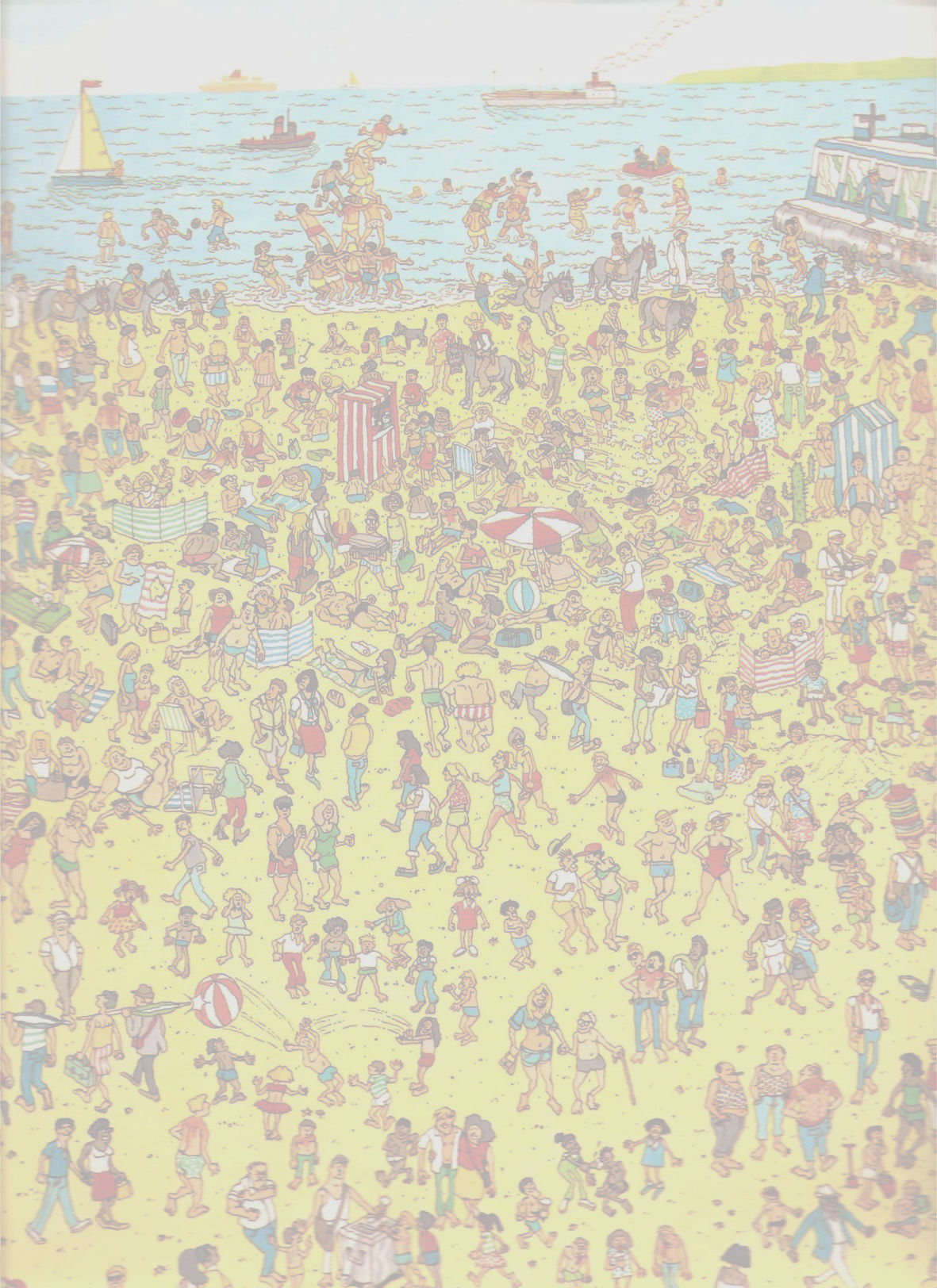
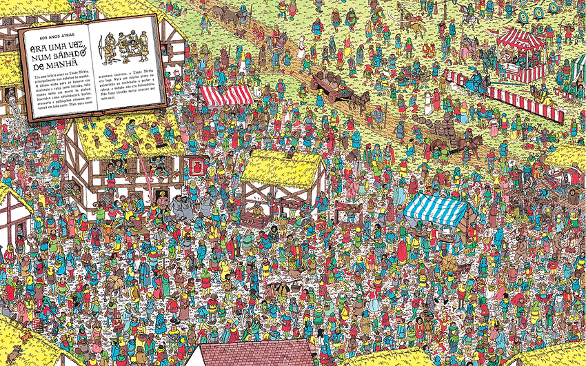
Below is the main code, referencing several functions that are illustrated in the following description. In order to demonstrate how the code works, we will be using the image in Figure 1 as our test example.

clear;

clc;

pic = input('Input an image name:', 's');

image = imread(pic);

[redImage, whiteImage] = extractRedAndWhite(image);

filteredImage = colorDependenceFilter(redImage, whiteImage);

[x,y] = stripeCorrelation(filteredImage);

%%Find Waldo

figure

imshow(image)

hold on

rectangle('Position',[x-100,y-100,200,200], 'LineWidth',5)

Figure 1: Test Example

Approach Overview

Function #1: Extract Red and White

In this function, the test image serves as the input, where it first identifies pixels of the image that are red using threshold values for each RGB value. Once those are identified, a "redImage" is generated that replaces all identified red pixels with white pixels and all nonred pixels are made black.

Using the same logic, in order to identify the white pixels in the image, threshold values are set for each RGB value. Once the white pixels are identified, "whiteImage" replaces all identified white pixels and keeps them white while making all other nonwhite pixels black.

function [ redImage, whiteImage ] = extractRedAndWhite( testImage )

%%Create an image keeping only the red portions of the input

keptValues = (testImage(:,:,1) > 150) & (testImage(:,:,2) < 100) & (testImage(:,:,3) < 100);

redImage = zeros(size(testImage));

[nf,nc]=size(testImage);

holder=ones(nf,nc)*255;

redImage(:,:) = holder(:,:).*[keptValues keptValues, keptValues];

%%Create an image keeping only the white portions of the input

whiteImage = zeros(size(testImage));

keptValues = (testImage(:,:,1) > 175) & (testImage(:,:,2) > 175) & (testImage(:,:,3) > 175);

whiteImage(:,:) = holder(:,:).*[keptValues keptValues, keptValues];

end

The figures below show the output of the redImage and whiteImage variables.

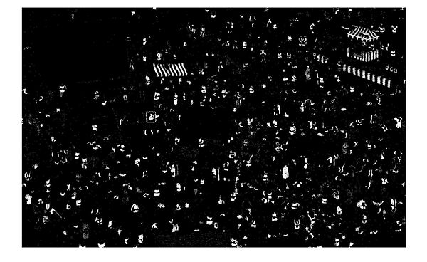
Figure 2: RedImage

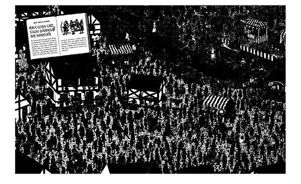
Figure 3: WhiteImage

Function #2: Color Dependence Filter

The purpose of this filter is to take the redImage and the whiteImage determined from the previous step, and iteratively filter out regions that do not have adjacent red and white pixels

This is done by first using a moving average filter to determine and highlight regions of red in the redImage, and the multiply it by the white image so that it eliminates white pixels that are far away from red areas.

Similarly, we use a moving average filter to determine and highlight regions of white pixels and apply the same method to eliminate red pixels that are far away from white areas.

function [ redImage ] = colorDependenceFilter( redImage, whiteImage )

%%Use the two images to iteratively filter out parts of the image that dont

%%have red or white

[nf,nc] = size(redImage);

redImage = rgb2gray(redImage);

whiteImage = rgb2gray(whiteImage);

AveFilter=ones(floor(nf/150),floor(nc/150));

for i=1:1

REDFILTERED=conv2(redImage,AveFilter);

auxvector=find(REDFILTERED<5);

REDFILTERED(auxvector)=0;

whiteImage = whiteImage.*REDFILTERED(1:nf,1:nc/3);

REDFILTERED=conv2(whiteImage,AveFilter);

auxvector=find(REDFILTERED<5);

REDFILTERED(auxvector)=0;

redImage = redImage.*REDFILTERED(1:nf,1:nc/3);

redImage(redImage > 0) = 1;

whiteImage(whiteImage > 0) = 1;

end

The figures below show the output of this filter.

Figure 4: Filtered Image

Function #3: Stripe Cross Correlation

The purpose of this filter is to take the filtered image from the previous step and cross correlate it with a 16 x 16 pixel black and white striped image.

function [ x,y ] = stripeCorrelation( redImage )

%%Generate a set of black and white stripes

testStripe = ones(16,16);

testStripe(1:4, :) = 0;

testStripe(9:12, :) = 0;

%%Correlate the stripes with the filtered image

test = normxcorr2(testStripe,redImage);

[y,x] = find(test==(max(max(test))));

end

The striped image is shown below.

Figure 5: 16 x 16 pixel Striped Image

The correlation surface is shown in the graph in Figure 6 as the peak value, which gives the x and y location of Waldo in Figure 7.

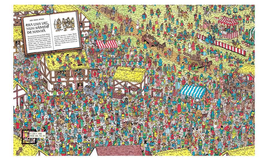
Figure 6: Correlation Surface with the location of the maximum value pointed out.

Figure 7: Location of Waldo based on peak value.

Figure 8: Zoomed in location of Waldo based on peak value.